A tutorial for running a flood simulation

This tutorial is written as a Jupyter notebook and provides a step-by-step tutorial for setting up a flood model and plot its outputs. We will use the sample data included in the pypims package. The notebook can be downloaded from Github.

Authors: Xilin Xia, Xiaodong Ming

Date: 21/10/2022

Explaining the data

The first step is to list which data is included in the sample.

from pypims import IO
import os
from pypims.IO.demo_functions import get_sample_data
dem_file, demo_data, data_path = get_sample_data() # get the path of sample data
os.listdir(data_path)

['landcover.gz', 'DEM.gz', 'rain_mask.gz', 'rain_source.csv']

As we can see from the list, there are 4 files in the folder. The three files ended with ‘.gz’ are raster files for the DEM, rainfall mask and land cover types. These files are gzip compressions of ArcGIS ASCII format. We used compressed format to save some space, but pypims can also read original ArcGIS ASCII or GeoTIFF formats. The other file named ‘rain_source.csv’ is the time series of the rainfall intensity. We will now load these files and explain what they are used for in the simulation.

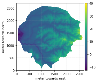
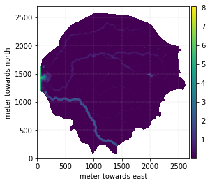
The first file we will look at is ‘DEM.gz’. It defines the topography on which the flood simulation is running. In the simulation, each single valid pixel in the DEM is a cell within the computational domain. We can use the ‘Raster’ and ‘mapshow’ functions built in pypims to visualise them. As we can see from the figure, the DEM represents a catchment with a main river ending in the sea.

DEM = IO.Raster(os.path.join(data_path,'DEM.gz')) # load the file into a Raster object
DEM.mapshow() # plot the Raster object

(<Figure size 432x288 with 2 Axes>,
 <AxesSubplot:xlabel='meter towards east', ylabel='meter towards north'>)

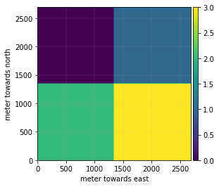
The other file ‘rain_mask’ gives an index (0, 1, 2, …) to every grid cell. These indices decide which column of the rainfall intensity time series will be used as the rainfall source term. As we can see from the figure, the domain has four different indices ‘0’, ‘1’, ‘2’, ‘3’.

rain_mask = IO.Raster(os.path.join(data_path,'rain_mask.gz'))
rain_mask.mapshow()

(<Figure size 432x288 with 2 Axes>,
 <AxesSubplot:xlabel='meter towards east', ylabel='meter towards north'>)

We can use the pandas package to load ‘rain_source.csv’ and show its contents. The first column is the time stamps (in seconds). The other columns are the rainfall intensity values (in meter per second) for cells with rain mask indices starting from 0. For instance, the second column is for cells with index 0, the third column is for cells with index 1 and so on.

import pandas as pd
rain_source = pd.read_csv(os.path.join(data_path,'rain_source.csv'), header = None)
rain_source.head()

	0	1	2	3	4
0	0	0	0.000014	0	0.000001
1	360	0	0.000014	0	0.000001
2	720	0	0.000014	0	0.000001
3	1080	0	0.000014	0	0.000001
4	1440	0	0.000014	0	0.000001

The file ‘landcover.gz’ gives difference indices to each grid cell to label their land cover types. In our case, there are two land cover types labelled by ‘0’ and ‘1’. We can use it as a reference to define parameters that are spatially variable.

landcover = IO.Raster(os.path.join(data_path,'landcover.gz'))
landcover.mapshow()

(<Figure size 432x288 with 2 Axes>,
 <AxesSubplot:xlabel='meter towards east', ylabel='meter towards north'>)

Generating the inputs and runing the simulation

We will now use the data we have just loaded to set up a flood model. In the first step, we need to initialise an InputHipims object with the DEM. We also want to specify the directory where the simulation is run and the number of devices we want to use. In this example, we will only use a single GPU, but pypims support multiple GPUs too.

ngpus = 1
case_folder = os.path.join(os.getcwd(), 'hipims_case') # define a case folder in the current directory
case_input = IO.InputHipims(DEM, num_of_sections=ngpus, case_folder=case_folder)

We can then put some water in the catchment by setting an initial depth. In our case, the initial water depth is 0 m across the catchment.

case_input.set_initial_condition('h0', 0.0)

We need to put some boundary conditions herein. We assume that there is a 100 m3/s dicharge from the upstream of the river, and depth at the downstream is fixed as 12.5 m. The locations of the boundaries can be defined by a few boxes that enclose the boundary sections. We simply need to define the coordinates of two opposite corners of the box, for instance, the upper left and bottom right coner points.

import numpy as np
box_upstream = np.array([[1427, 195],  # bottom left
                         [1446, 243]]) # upper right
box_downstream = np.array([[58, 1645], # upper left
                           [72, 1170]]) # bottom right
discharge_values = np.array([[0, 100], # first column: time - s; second colum: discharge - m3/s
                            [3600,100]])

We then use a list of dicts to put things together.

bound_list = [
            {'polyPoints': box_upstream,
             'type': 'open',
             'hU': discharge_values},
            {'polyPoints': box_downstream,
             'type': 'open',
             'h': np.array([[0, 5],
                            [3600,5]])}] # we fix the downstream depth as 12.5 m

Now we can set up the boundary conditions and check whether they have been set up correctly.

case_input.set_boundary_condition(boundary_list=bound_list)
case_input.domain_show() # show domain map

Flow series on boundary 1 is converted to velocities
Theta = 135.00degree

(<Figure size 432x288 with 2 Axes>,
 <AxesSubplot:title={'center':'Domain Map'}, xlabel='meter towards east', ylabel='meter towards north'>)

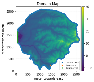
Great, the boundary conditions are set up correctly! We now need to setup the rainfall mask and rainfall time series.

rain_source_np = rain_source.to_numpy()
case_input.set_rainfall(rain_mask=rain_mask, rain_source=rain_source_np)

We also need to set up values for the Manning’s n. We can use the landcover map to define a spatially variable Manning’s n.

case_input.set_landcover(landcover)
case_input.set_grid_parameter(manning={'param_value': [0.035, 0.055],
                                        'land_value': [0, 1],
                                        'default_value':0.035})

We want to see the time histories of the depth at both the downstream and upstream of the main river, so we need to set up a gauging point in the model.

case_input.set_gauges_position(np.array([[560, 1030],
                                        [1140,330]]))

The final thing we want to set up is the runtime. We want to run the simulation for 2 hours, get the raster outpurs for every 15 minutes and backup the simulation for every half an hour.

case_input.set_runtime([0, 7200, 900, 1800])

'0-start, 7200-end, 900-output interval, 1800-backup interval'

We have now finished setting up the model. Let’s see what the model summary tells us.

print(case_input)

---------------------- Model information ---------------------
case_folder : pypims/source/Tutorials/hipims_case
birthday : 2021-10-27 00:23
num_GPU : 1
run_time : [0, 7200, 900, 1800]
num_gauges : 2
---------------------- Grid information ----------------------
area : [4351200.0, 'm^2']
shape : (269, 269)
cellsize : [10.0, 'm']
num_cells : 43512
extent : {'left': 0.0, 'right': 2690.0, 'bottom': 0.0, 'top': 2690.0}
---------------------- Initial condition ---------------------
h0 : 0.0
hU0x : 0
hU0y : 0
---------------------- Boundary condition --------------------
num_boundary : 3
boundary_details : ['0. (outline) fall, h and hU fixed as zero, number of cells: 788', '1. open, hU given, number of cells: 2', '2. open, h given, number of cells: 46']
---------------------- Rainfall ------------------------------
num_source : 4
max : [50.0, 'mm/h']
sum : [12.38, 'mm']
average : [13.75, 'mm/h']
spatial_res : [924.0, 'm']
temporal_res : [360.0, 's']
---------------------- Parameters ----------------------------
manning : [[0.035, 0.055], '[72.92, 27.08]%']
sewer_sink : 0
cumulative_depth : 0
hydraulic_conductivity : 0
capillary_head : 0
water_content_diff : 0
InputHipims object created on 2021-10-27 00:23:00

All seems to be good. We can now write these inputs into files that the flood simulation engine reads.

case_input.write_input_files()

/media/data/lunet/cvxx/hipims_python/docs/source/Tutorials/hipims_case/input/mesh/DEM.txt created
times_setup.dat created
device_setup.dat created
z created
h created
hU created
precipitation created
manning created
sewer_sink created
cumulative_depth created
hydraulic_conductivity created
capillary_head created
water_content_diff created
precipitation_mask created
precipitation_source_all.dat created
boundary condition files created
gauges_pos.dat created

Let’s run the model now. It will show ‘Simulation successfully finished’ if the simulation finishes without an error.

from pypims import flood
if ngpus > 1:
    flood.run_mgpus(case_folder)
else:
    flood.run(case_folder)

...
Simulation successfully finished!
Writing output files
Writing backup files
Writing maximum inundated depth.
Total runtime 5410.26ms

Plotting the results

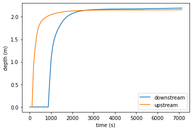
After the simulation finishes, we can plot the depth at the gauge point and the maximum inundation depth over the domain. To do this, we need to create an OutputHipims object first.

case_output = IO.OutputHipims(input_obj = case_input)

Then we can read the depth from the outputs.

gauges_pos, times, values = case_output.read_gauges_file(file_tag = 'h')

After reading the output into numpy arrays, we can use matplotlib package to plot the depths at the gauge points.

import matplotlib.pyplot as plt
lines = plt.plot(times, values)
plt.xlabel('time (s)')
plt.ylabel('depth (m)')
plt.legend(lines[:2],['downstream','upstream'])
plt.show()

We can also use pypims to read the raster outpus and use mapshow to show the results.

max_depth = case_output.read_grid_file(file_tag='h_max_7200')
max_depth.mapshow()

(<Figure size 432x288 with 2 Axes>,
 <AxesSubplot:xlabel='meter towards east', ylabel='meter towards north'>)

Pypims only provides some basic functions for visualising the outputs. If you need to plot something more beautiful for your reports or papers, the matplotlib package is a good place to start with.

Hope you have enjoyed reading this tutorial. Please dive into the API documentation for more advanced usage of pypims.